
Aerodynamics of An Ahmed Body
We want to simulate the flow around a simplified car geometry, known as Ahmed body. The quantity of interest is the aerodynamic drag force.
Model validation is based on the experimental data of Ahmed et al. (1984).
After generating a mesh of 500,000 cells (Fiigure 1). A body of influence allow local mesh refinement in the wake to capture the flow details. Inflation is also used next the body surface to capture the boundary layer.

Figure 1: poly-hexcore mesh with a BOI
The velocity magnitude field over the Ahmed Body model is shown at different planes in Figure 2.
The rear of the body presents a recirculation region, the low velocity continues downstream.

Figure 2: Velocity magnitude contours at side and top views.
The velocity magnitude field over the Ahmed Body model is shown at different planes in Figure 3.
It shows a high pressure region in the leading edge of the body and low pressure at the slopes of the body and in the wake also.

Figure 3: Static pressure contours at side and top views.
In essence, the pressure difference between the front and the rear of the body is the main cause for the drag (pressure drag).
Speaking of which, the numerical drag coefficient equals 0.21 while the experiments gave 0.28 for the same slant angle
Flow past
cylinder
We want to simulate the unsteady dynalics of the flow around a solid cylinder, in 3D, using a transient time formulation. The quantities of interest are the aerodynamic forces of drag and lift.
The aim of this time-dependent study is to infer the dominant oscillation frequency or the strouhal number St of the unsteady flow.
For this case, an unstructured triangular mesh is generated. Sweep method is used to impose a 1 cell thickness in the cylinder axis direction. A body of influence allow to capture the near wake physics and the boundary layer is resolved (y+<1)
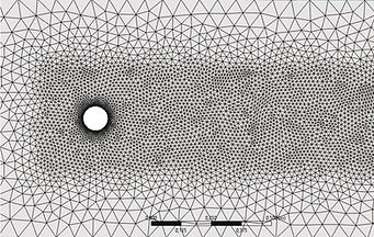
Figure 1: Sweep triangular mesh with a BOI
For time resolution, a fixed time step is used to keep a CFL <10, the physical flow time is 60 seconds.
Animation 1: unsteady flow contours at Re=1000. (L) Velocity magnitude. (R) Pressure.

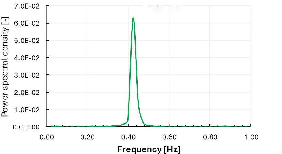
Figure 2: Spectral density of drag and lift using FFT
The contours of the flow variables (Animation 1), show a periodic vortex shedding regime characterized by a turbulent wake.
Thanks to the spectral analysis shown in Figure 2, the dominant frequency of drag is twice that of lift and the Strouhal number equals 0.22
Z bend
Mixing
We want to simulate heat transfer of the internal flow in a Z bend in the steady state.
The design study was carried as part of a simulation challenge for my application to the start up Zelin. The Z shaped bend is in fact their logo.
The unstructured mesh is composed of tetrahedral elements. Surface sizing at the elbows. 3 meshes of: 35k, 75k and 145k cells were generated to perform a grid independance test. The boundary layer is not resolved (y+=45).
There is no significant effect on the solution, starting from 75 k cells.

Figure 1: Cross section of tetra mesh with 75k cells
A global time-step approach is preferred to solve the flow (pseudo-transient).
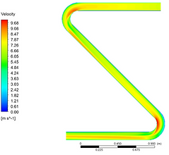
Figure 2: velocity magnitude contour at mid-plane

Figure 3: static pressure contour at mid-plane
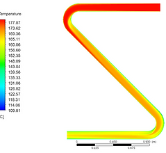
Figure 4: Temperature contour at mid-plane
The heat transfer corresponds to the heat loss at the bend walls from natural convection with the ambient air.
An approximation of the flow dynamics is by treating flow variables as passive scalars. Thus, the physical characteristics of the fluid such as: density, viscosity, thermal conductivity, stay constant.
Turbomachinery: centrifugal pump
We want to simulate the rotating flow in the centrifugal pump impeller-volute bodies.
An MRF (Multiple reference Frame) is applied by considering the relative motion in the moving region (impeller at 1500 rpm). From now on we denote impeller as rotor, and volute as stator.
To gain a considerable computational cost, periodic boundary conditions come in handy. Thus, 1/6 of the rotor is modelled corresponding to 1 blade thanks to rotational symmetry.
The grid consists of polyhedral elements. The boundary layer is accounted for using last ratio method, using 3 prism layers. After testing the independence of the mesh, we pick a medium grid with 240k cells. Face sizing is used to match interfaces.
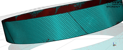
Figure 1: Mesh interface rotor-stator
In the solver, we set a mesh interface rotor-stator with no-pitch scale as shown in Figure 1. Since we generated the missing instances by symmetry.
A global time-step approach is preferred to solve the flow (pseudo-transient).

Figure 2: Flow variables contours at mid-plane for Q=80 Kg/s.
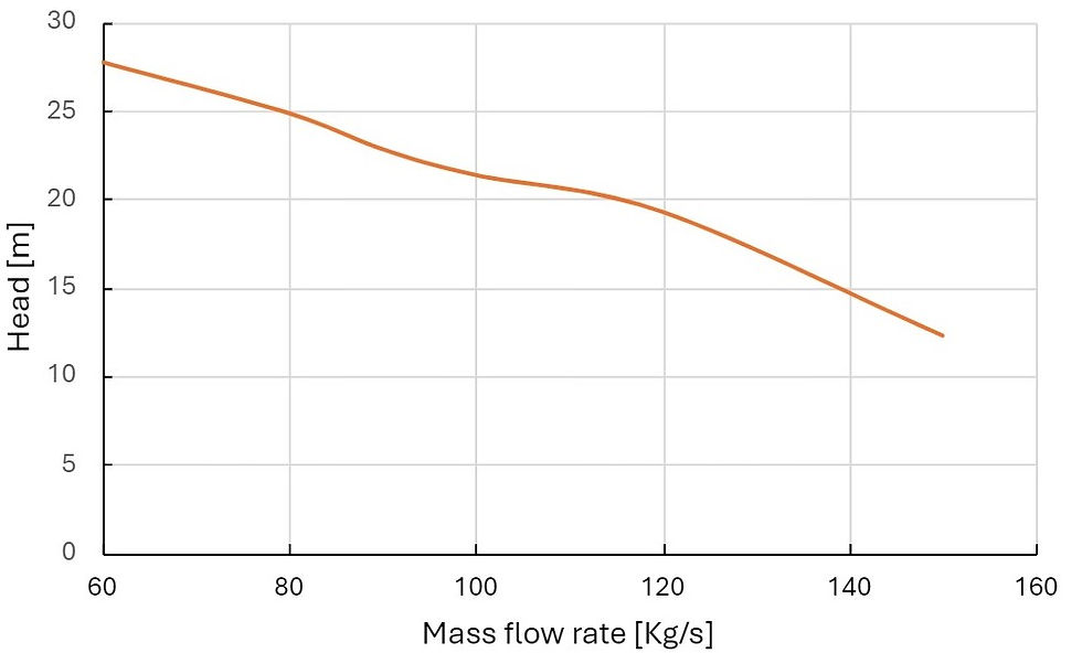

Figure 3: Pump characteristics against the mass flow rate.
Figure 2 contours show that the near center region is more vulnerable to cavitation since it represents a low pressure zone (below 1 bar) susceptible to fall under the saturation pressure value if the rate of rotation is increased.
The pump characteristics indicate an optimal efficiency of 89% at approximately Q=85 Kg/s corresponding to a head of 24 m.
Internal flow of a globe valve
We aim to simulate the internal flow in a globe valve with its complex features. The idea is create as many geometries as the lift positions considered for the valve plug. Which mimics a simulation of a dynamical system.
The CAD in this case has some features that are superfluous from a CFD analysis point of view. Therefore, they're removed in the geometry clean-up and the volume flowing in the valve is extracted.
As mentioned earlier, we have to mesh each lift instance of the geometry. An unstructured grid of polyhedral elements is created with Fluent 3D mesher. A facesizing is used on the plug walls to capture small details that may influence the flow. The boundary layer is accounted for using smooth transition method, using 5 prism layers.
Grids of approximately 0.3 M cells are generated for the range of lift positions [1, 5, 10, 20] mm.

Figure 1: Polyhydra mesh with facesizing on plug
We set 3 different operating conditions with respect to inlet pressure : 4, 5, 8 bars respectively. While outlet is kept at constant pressure of 3 bar.
Standard steady formulation is picked for time resolution (no pseudo-time stepping)

Figure 2: Flow variables contours at mid-plane for varying lifts; Δp: 1 bar (top), 2 bar (bottom left), 5 bar (bottom right)
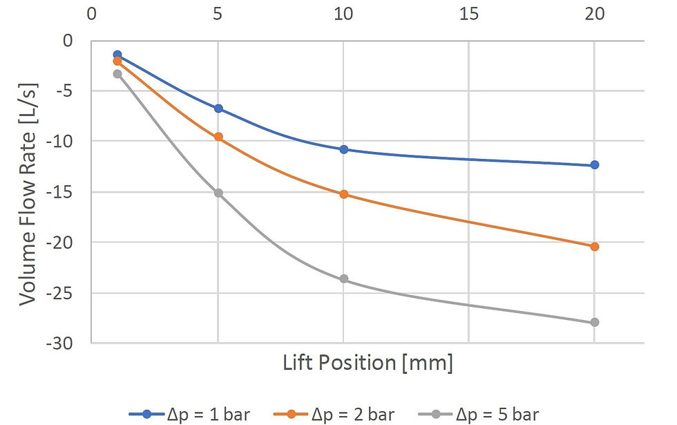
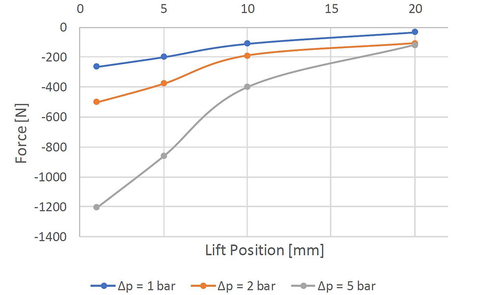
Figure 3: Valve characteristics against the lift positions.
Pressure contours shown in Figure 2 give an insight to the hydraulic load on the disc. As the plug is lifted, pressure distribution is more and more homogeneous between the two compartments, hence, more upward force is applied.
This observation is confirmed quantitatively with the curves of vertical force of Figure 3. Since the required force for valve lift tends towards zero as we move towards a fully lifted position.
Based on characteristic curves at different operating conditions, we inferr fast opening performance of this globe valve.